Excel’s power is all in the formulas.
Without formulas, Excel is a semi-automated calculator with a keyboard. With formulas, Excel becomes a paragon of automated data processing. When used well, Excel can load, parse, transform, update, create, and calculate nearly anything.
Formulas are the key that unlocks Excel’s capabilities. For new users, the mechanics of how formulas work and which to use can seem overwhelming. In this guide, we’ll start by reviewing the basics of how to build formulas. We’ll then dig into the handful of formulas that you’ll need to solve ninety percent of your Excel problems.
Formulas Cheat Sheet
Function Keys
- Toggle Enter/Edit Mode:
F2 - Toggle Reference Modes:
F4
Basic Operators
Formula Punctuation
- Identifying a formula:
= - Defining ranges:
: - Separating terms:
, - Grouping terms:
()
Comparison Operators
- Checking for equality:
= - Checking for inequality:
<> - Greater than, greater or equal, less than, less or equal:
>,=>,<,<=
Arithmetic Operators
- Addition:
+ - Subtraction:
- - Multiplication:
* - Division:
/
Text Operators
- Identifying text:
"" - Concatenation:
&
Aggregation
- Minimum:
MIN() - Maximum:
MAX() - Count numbers:
COUNT() - Count all items:
COUNTA() - Sum a range:
SUM() - Average a range:
AVERAGE()
Conditionals
- If statements:
IF() - Count numbers if a set of conditions are met:
COUNTIFS() - Sum a range if a set of conditions are met:
SUMIFS() - Average a range if a set of conditions are met:
AVERAGEIFS()
Matching & Search
- Find the value at a certain location:
INDEX() - Search a range:
MATCH()
Function Keys
Toggle Enter/Edit Mode: F2
F2 is the most useful keyboard shortcut in Excel. It toggles your keyboard’s input mode between Enter Mode and Edit Mode. What does that mean? Great question!
The bottom left corner of the Excel window displays your input mode
If you’ve used Excel then chances are you’ve edited a formula. For most people this means moving your hands off of the keyboard, grabbing your mouse, moving your cursor to the formula bar, clicking into the formula in the right place, and moving your hands back to the keyboard.
This doesn’t sound too inefficient but over time it adds up. Constantly switching between your mouse and keyboard is a huge drain on productivity and focus. Think of it like the Excel version of hunt and peck typing.
Luckily, there’s a solution — F2 allows us to edit cells without our hands ever leaving the keyboard!
If you select a cell and press F2, then you immediately flip into Edit Mode for that cell. Pressing left or right on the arrow keys will move the cursor within the cell’s formula. Typing will change the contents. While editing, press Enter to save your changes or Esc to cancel them.
Excel also lets you switch between input modes while editing a formula. While in Edit Mode, if you place your cursor before or after an operator (e.g.: +, -, &) and press F2, you will switch to *Enter Mode. *This lets you use your arrow keys to insert a new cell reference at that place.
Note that using the arrow keys to add a cell reference only works if your cursor is before or after an operator. In other words, your cursor must be somewhere in the formula where it makes sense to add a cell reference. If it isn’t then using the arrow keys will close the cell.
Using F2 to edit cells makes it very easy to update your formulas without time spent hunting and pecking.
Toggle Reference Modes: F4
F4 allows us to toggle between cell reference modes while editing formulas.
To use F4, click into a formula so that your cursor is touching a cell reference (e.g.: A1 or C7). When you press F4 you will see some dollar signs appear around the cell name. These dollar signs show when that part of the cell reference locks. Continuing to press F4 will toggle between four settings:
- Locking row and column:
$A$1 - Locking row only:
A$1 - Locking column only:
$A1 - Unlocked:
A1

If you aren’t sure why this is useful don’t worry, we’ll go over the uses in detail in the next article, Formula Construction.
Basic Operators
Formula Punctuation
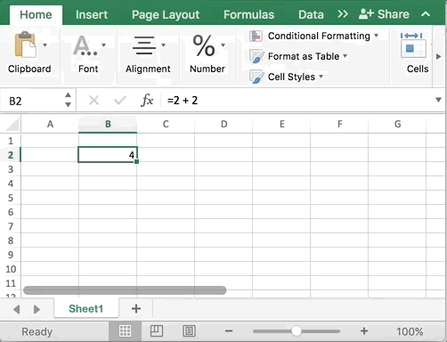
Identifying a formula: =
All formulas in Excel must start with a = sign. This symbol tells Excel that it should calculate the cell. If you do not include the = sign, then that cell will display as text instead.
Defining ranges: :
The : operator allows us to define ranges in formulas. Ranges are defined by a starting cell and an ending cell joined together with a :. For example, the range A1:B2 includes the cells A1, A2, B1, and B2. Ranges defined with the : operator have a few rules:
- They are continuous (there’s no way to exclude a cell in the middle of the range)
- The first cell reference in the formula must be in the upper left of the range
- The last cell reference in the formula must be in the lower right of the range
To make a range that spans an entire column leave off the numbers (e.g.: A:A). To make a range that spans an entire row leave off the letters (e.g.: 1:1).
Separating terms: ,
Some formulas like IF() statements need a few separate pieces of information. The , operator lets us tell Excel when one section has ended and the next begins. The pieces of a formula are often called “arguments”, “parameters”, or “terms.” These terms are interchangeable.
Grouping terms: ()
Use parentheses to define the order of operations in your formulas. Like any arithmetic formula, It will calculate any items inside parentheses first.
Comparison Operators
Checking for equality: =
Besides indicating a new formula, we can use the equals sign to check for equality. For example, =2 = 2 is a formula to check whether the value 2equals the value 2. Since these two values are the same, the cell’s result will be TRUE.
Checking for inequality: <>
Using <> between two items within a formula will check if those items are not equal to each other.
Greater than, greater or equal, less than, less or equal: >, =>, <, <=
These operators compare two items together and return a TRUE or FALSE result.
Arithmetic Operators
I’m going to go out on a limb and say that these don’t need too much explanation.
Text Operators
Identifying text: ""
Wrapping something in quotes tells Excel to treat that section as plain text (i.e.: not an item to calculate). Snippets of text inside quotes are often called “strings.”
Concatenation: &
Putting the concatenation operator & between two strings of text joins those strings together. A common use case for this operation is joining together first and last names. Keep in mind that the operator will join the two strings exactly. If you want a space between items you will have to add it manually.
Note that using the & operator will also work with numbers. Be careful though, concatenating numbers is risky! It will attach the numbers together instead of adding them. This is hard to follow can lead to many frustrated hours of debugging when your results don’t look like you expect.
Aggregation
Minimum: MIN()
=MIN(number1, [number2], ...)
Use this function to find the lowest number in a list of numbers. The numbers can be cell references, ranges, or a combination of the two. Any text referenced within the formula will be ignored when the formula calculates.
Maximum: MAX()
=MAX(number1, [number2], ...)
This formula is exactly like MIN() but it finds the largest number in the series instead of the smallest.
Count numbers: COUNT()
=COUNT(value1, [value2], ...)
The COUNT() formula returns the amount of numbers within the range you define. Like MIN() and MAX(), you can define the range in a few ways. This function will ignore any non-number values.
Count all items: COUNTA()
=COUNTA(value1, [value2], ...)
Like COUNT(), this formula will return the amount of numbers within a range. Unlike COUNT(), this formula will also count any non-numeric values. This can be great in most cases but be careful you don’t include titles in your range!
Sum a range: SUM()
=SUM(number1, [number2], ...)
This formula is a convenience function. It exists so that when summing many cells we don’t have to list them individually with a string of +s. Like MIN(), MAX(), and COUNT() you can define the range to sum in a variety of ways. Any text included in the range will be ignored.
Average a range: AVERAGE()
=AVERAGE(number1, [number2], ...)
Much like SUM(), this will return the average of whatever range of numbers you put in. It will also ignore any text inside of the range you define.
Conditionals
If statements: IF()
=IF(logical test, value if true, [value if false])
Learning to use IF() functions well is one of the biggest force multipliers in Excel. Unlike the formulas we’ve gone over so far IF() statements have a few terms. When writing the formula, separate each term from its neighbors with a comma.
The first term needs to be some kind of logical test that gives TRUE or FALSE as a result. A very simple example is 1 = 1 but depending on your needs they could be much more complex. Often times you will use an IF formula to check if another cell equals a certain value. In this case, your first term would be something like A1 = "some specific string".
The second and third terms are what you want your cell to display. Which one appears depends on the result of the logical test in your first term. If your logical test evaluates to TRUE then Excel will display whatever is in your second term. If your logical test evaluates to FALSE then Excel will display whatever is in your third term. These could be simple values like "it was true", "it was false", or 385 or formulas in their own right.
For example, let’s say you want to check whether cell A1 equals the string apple. If it does, you want to display cell B1 which holds the value fruit. If it is false, you want to display cell B2 which holds the value not a fruit. The IF() formula you would need is below:
Count numbers if a set of conditions are met: COUNTIFS()
=COUNTIFS(criteria range1, criteria1, ...)
Often we will want to take the count of a range subject to a certain condition. For example, “count the numbers in column A where column B is TRUE.” Excel actually has two formulas that can do this: COUNTIF() *and *COUNTIFS(). The difference between the two is that COUNTIFS() (with an extra S) works with one or more conditions. Rather than remembering two sets of syntax, default to using COUNTIFS(). The items in the COUNTIFS() formula must come in pairs. The first item is the range you’d like to count, the second is the criteria for which items to include and exclude. If you wanted to count column A where the value was TRUE then the formula would be:
=COUNTIFS(A:A, TRUE)
To add more criteria, say where column B is the number 6, add another term:
=COUNTIFS(A:A, TRUE, B:B, 6)
This will return the count of rows where column A is TRUE and where column B is 6. If one or the other of those checks is false that row will not be included in the count. Make sure that the ranges you use are all the same size. If they are not, then the formula will not be able to compare across each range and the formula will return a#VALUE! error.
Sum a range if a set of conditions are met: SUMIFS()
=SUMIFS(sum range, criteria range1, criteria1, ...)
Like COUNTIFS(), SUMIFS() is like the SUM() formula plus conditions. Unlike COUNTIFS() you’ll have to tell Excel which range you want to sum too. The range to sum is the first term in the formula. After defining the range to sum you can add as many range and condition pairs as you need. Summing column A based on conditions in columns B and C would look like this:
=SUMIFS(A:A, B:B, TRUE, C:C, 6)
Average a range if a set of conditions are met: AVERAGEIFS()
=AVERAGEIFS(average range, criteria range1, criteria1, ...)
The construction and use of AVERAGEIFS() is exactly the same as SUMIFS(). It also needs a range to average as the first term and then criteria and criteria ranges afterward. A formula to average row 1 based on the values in row 2 and 3 might look something like this:
=SUMIFS(1:1, 2:2, TRUE, 3:3, 6)
Matching & Search
Find the value at a certain location: INDEX()
=INDEX(array, row num, [column num])
The simplest form of INDEX() takes a range and a number as inputs. In the background, the formula starts at the upper left corner of your range. It then counts down the number of cells you tell it using the second argument and returns the value in that cell.
=INDEX(A:A, 5) → whatever the value is in A5
You can also add a second term to count to the right as well.
=INDEX(A:D, 1, 3) → whatever the value is in C1
Search a range: MATCH()
=MATCH(lookup value, lookup array, [match type])
MATCH() is a search function. The first argument is the item you’d like to search for, and the second term is the range where you’d like to search). An important thing to know about MATCH() is that its main purpose is to find numbers, not text. This is why there is a third term, match type, that in most cases we will have to enter.
If we want to find a number that’s greater than or equal to our search value then we enter -1 for the third term. If we want a value that’s less than or equal to our search term, we enter 1 or leave the field blank (this is the default). If we want to find an exact match, the third term should be 0.
As you might imagine, this works much better with numbers than it does with text. If you use MATCH() with text make sure that your third term is always 0.
MATCH() returns the index of the first cell where it finds a value that matches your search criteria. For example, if the string some string is in cell A4, then the formula would return 4.
=MATCH("some string", A:A, 0) → 4
Matching cells: VLOOKUP(), HLOOKUP()
If you’ve ever heard anyone brag about their Excel skills then you’ve likely heard of VLOOKUP(). Considering how core a tool VLOOKUP() (and it’s cousin, HLOOKUP()) is for most people you’re probably surprised it isn’t on this list.
It isn’t here because it’s awful.
They’re inefficient, rigid, and most importantly, prone to breaking silently. Whether someone cringes at the mention of VOOLKUP() is one litmus test for how well they know Excel. Serious Excel users know that there’s a much better way to match cells with INDEX() and MATCH(). We’ll go over the details and more in the next article in this series — Formula Construction.